Information about using the make_energy_vs_similarity_results.py script
This page gives a description how to analysed the clusters that have been created. This page is an extention of make_energy_vs_similarity_results.py - For analysing the genetic algorithm under-the-hood
One of the bits of information that you may like to obtain from the genetic algorithm, especially if you are accessing the efficiency of the genetic algorithm program, is what happened when various genetic algorithms ran. One way of assessing what happened during a genetic algorithm is to observe what clusters were created as the genetic algorithm ran. This is practically very hard to do if you are just looking at the clusters that are made. However, if you can assess the clusters that you make with various parameters, you can get a better idea of the type of clusters that were created during your genetic algorithm.
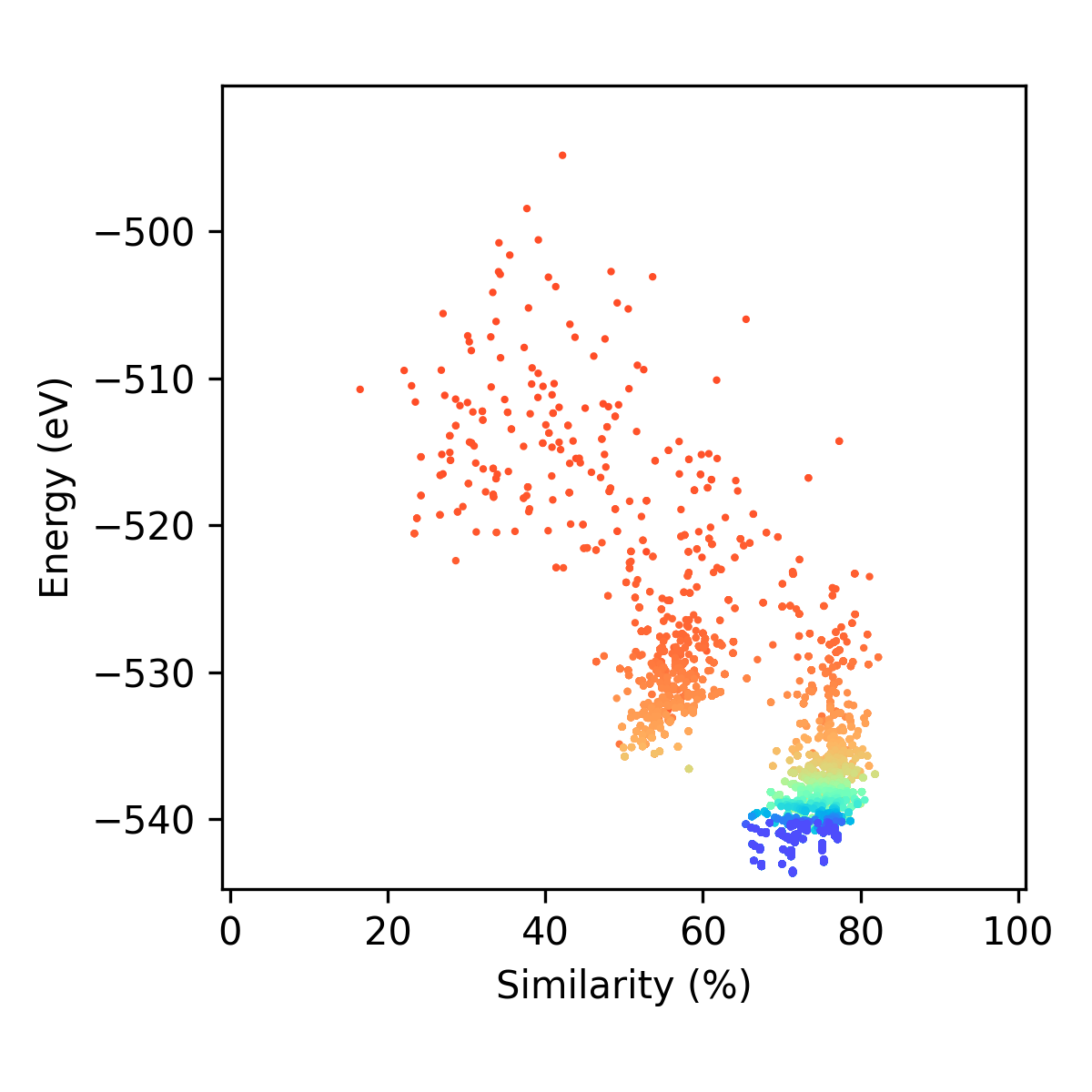
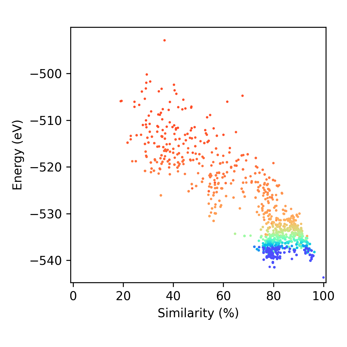
The best way to monitor the types of clusters that are created is using a potential energy surface (PES) plot, which describes the energy as a function of the spatial positions of the atoms in your cluster. This type of plot can not be visualise as this would require a plot with \(3N-6\) spatial axes and one energy axis (where \(N\) is the number of atoms in your cluster). Instead, we (and others in the literature) have found it best to replace the \(3N-6\) spatial axes with one or two axis that describe the structural similarity between clusters.
In Organisms, we have a function that is able to describe the structural similarity between various clusters based on the common neighbour analysis. This function is called the Structural Comparison Method (SCM). Using this similarity parameter, it is possible to plot a PES plot, where:
the x axis is the similarity between clusters made during your genetic algorithm against a reference cluster, and
the y axis is the energy of the cluster.
We have created the make_energy_vs_similarity_results.py program that processes the data from your genetic algorithm and gives you energy vs. similarity plots that describes the types of cluster that were created during the genetic algorithm and plots them in the style of a PES plot. In this page, we will describe how to use this program, as well as describe the types of plots that you will obtain from this program.
See Development of a Structural Comparison Method to Promote Exploration of the Potential Energy Surface in the Global Optimisation of Nanoclusters; Geoffrey R. Weal, Samantha M. McIntyre, and Anna L. Garden; JCIM; DOI: 10.1021/acs.jcim.0c01128 for more information about how these energy vs similarity plots can be used to help you understand how the Organisms genetic algorithm program is running.
Requirements for using the make_energy_vs_similarity_results.py Program
To use this program, you must record all the clusters that were created during the genetic algorithm. This requires your ga_recording_information dictionary to be set to record all clusters created during the genetic algorithm. Do to this, include the following in the ga_recording_information variable in your Run.py file:
ga_recording_information = {}
ga_recording_information['ga_recording_scheme'] = 'All'
ga_recording_information['exclude_recording_cluster_screened_by_diversity_scheme'] = False
Note that you can still set the saving_points_of_GA, record_initial_population, and show_GA_Recording_Database_check_percentage variables how ever you like.
Running the make_energy_vs_similarity_results.py Program
Due to the complexity of the information required to run this program, this program is executed from a python script rather than accessing it directly unlike most of the other side programs available in Organisms.
An example of the Run_energy_vs_similarity_script.py script that is used to execute the make_energy_vs_similarity_results.py program for a global optimisation of a 98-atom Lennard-Jones cluster is given below:
 1from ase.io import read
 2from asap3.Internal.BuiltinPotentials import LennardJones
 3from Organisms import make_energy_vs_similarity_results
 4
 5# ===========================================================================================================
 6# Information for processing data
 7#
 8# The path to where the genetic algorithm was run from (the directory where Run.py is found).
 9path_to_ga_trial = '.'
10# The rCut value for the common neighbour analysis, in units of Angstroms
11rCut = 1.355 # Angstroms
12# The ase.Atoms object of the cluster to compare all clusters from the genetic algorithm to.
13# In this example, we are comparing all clusters to the LJ98 global minimum.
14clusters_to_compare_against = read('LJ98_GM.xyz')
15# This is the calculator used to initially locally minimise ONLY the clusters_to_compare_against cluster
16# just to make sure this cluster is a local minimum.
17elements = [10]; epsilon = [1]; sigma = [1]; rCut_for_LJ_potential = 1000
18calculator = LennardJones(elements, epsilon, sigma, rCut=rCut_for_LJ_potential, modified=True)
19# Specify the number of cores you want to use.
20no_of_cpus = 1
21# ===========================================================================================================
22
23# ===========================================================================================================
24# Information for plotting data
25#
26# This setting will create plots that plot the energy vs similarity over generations, including generation plots of the eras between epoches.
27# This setting requires process_over_generations = True to be used.
28make_epoch_plots = True
29# This setting will create a video that shows how clusters were created per generations.
30# This setting requires process_over_generations = True to be used.
31get_animations = True
32# This setting will create a video that shows only the energies and similarities of clusters in the population over generation.
33# This setting requires process_over_generations = True to be used.
34get_animations_do_not_include_offspring = True
35# You can customise the unit that you give for the energy scale. For example, if you are wanting to obtain energy vs similarity plots for Lennard-Jones clusters, you may want to set this to 'LJ energy units'
36energy_units = 'LJ energy units'
37# This setting will indicate if you want to make svg files along with the png files that are made during this program
38make_svg_files = False
39# This is the number of generations that will be shown per second (gps) in your animation (if you choose to make animations of your genetic algorithm run.)
40gps = 60
41# You can also set the maximum amount of time that you would like your movie to run in minutes. You only need to give a value either for gps or max_time.
42max_time = None
43# You can include a label in your animations that will count the number of genrations that have past
44label_generation_no = True
45# You can include a label in your animations that will count the number of times an epoch occurs, i.e. will indicate the era value during the genetic algorithm
46label_no_of_epochs = True
47# place all these settings into the plotting_settings dictionary.
48plotting_settings = {'make_epoch_plots': make_epoch_plots, 'get_animations': get_animations, 'get_animations_do_not_include_offspring': get_animations_do_not_include_offspring, 'energy_units': energy_units, 'make_svg_files': make_svg_files, 'gps': gps, 'max_time': max_time, 'label_generation_no': label_generation_no, 'label_no_of_epochs': label_no_of_epochs}
49# ===========================================================================================================
50
51# ===========================================================================================================
52# Run the make_energy_vs_similarity_results program
53make_energy_vs_similarity_results(path_to_ga_trial, rCut, clusters_to_compare_against, calculator, no_of_cpus=no_of_cpus, plotting_settings=plotting_settings)
54# ===========================================================================================================
Lets go through each part of the Run_energy_vs_similarity_script.py file one by one to understand how to use it.
1) Variables for processing data
There are three variables required that determine how data from the genetic algorithm will be processed for making energy vs similarity plots. These are:
path_to_ga_trial (str.): This is the path to the genetic algorithm data that you want to process. This will have the same path as your
Run.pyfile.- rCut (float): This is the rCut value for the common neighbour analysis in Angstroms. This value determines which pairs of atoms are within bonding distance:
If a pair of atoms have an interatomic distance less than or equal to rCut, that pair of atoms is considered neighbours/bonded.
If a pair of atoms have an interatomic distance greater than rCut, that pair of atoms is not considered neighbours/bonded.
clusters_to_compare_against (ase.Atoms or [list of ase.Atoms]): These are all the clusters that you want to compare clusters to. Generally, you will only want to compared to genetic algorithm clusters to one reference cluster, such as the global minimum. However, if you need to do some checks, you can compare your genetic algorithm clusters to a few reference clusters. If you only want to give one reference cluster, assign clusters_to_compare_against to the
ase.Atomsobject for your cluster. If you have several reference clusters, put theirase.Atomsobjects into a list. You can import most types of files asase.Atomsobject using the ase.io.read function. See File input and output to read more about the read function in ASE.calculator (ase calculator): If you want to locally minimise the cluster you gave for clusters_to_compare_against before this algorithms begins, set the calculator to the calculator you used in your genetic algorithm. This will not locally minimise any of the clusters that you created during the genetic algorithm, it will only be used to locally minimise clusters_to_compare_against. If you set the calculator to
None, clusters_to_compare_against will not be locally optimised and will be used as is in this program. Default:Noneno_of_cpus (int): This is the number of cpus that are used to gather information that is used for making these energy vs similarity plots. Default:
1
An example of these parameters in Run.py is given below:
 5# ===========================================================================================================
 6# Information for processing data
 7#
 8# The path to where the genetic algorithm was run from (the directory where Run.py is found).
 9path_to_ga_trial = '.'
10# The rCut value for the common neighbour analysis, in units of Angstroms
11rCut = 1.355 # Angstroms
12# The ase.Atoms object of the cluster to compare all clusters from the genetic algorithm to.
13# In this example, we are comparing all clusters to the LJ98 global minimum.
14clusters_to_compare_against = read('LJ98_GM.xyz')
15# This is the calculator used to initially locally minimise ONLY the clusters_to_compare_against cluster
16# just to make sure this cluster is a local minimum.
17elements = [10]; epsilon = [1]; sigma = [1]; rCut_for_LJ_potential = 1000
18calculator = LennardJones(elements, epsilon, sigma, rCut=rCut_for_LJ_potential, modified=True)
19# Specify the number of cores you want to use.
20no_of_cpus = 1
21# ===========================================================================================================
2) Variables for plotting data
There are several variables required that determine how data from the genetic algorithm will be processed for making energy vs similarity plots. These are placed in the plotting_settings dictionary. These avariables are:
make_epoch_plots (bool): This plots the genetic algorithm over generations, as well as making plots over generations that are divided into era between epoches. Default =
False.get_animations (bool): This will make a movie file of your energy vs similarity plots as they were made over generations if you set this to
True. The offspring are included in this video. If you dont want these videos, set this toFalse. Default =False.get_animations_do_not_include_offspring (bool): This will make a movie file of your energy vs similarity plots as they were made over generations if you set this to
True. The offspring are not included in this video. If you dont want these videos, set this toFalse. Default =False.energy_units (str.): This variable allows you to give a custom unit for the energy the energy of your clusters are recorded in a units that is not eV. For example, if you are perfomring these plots on Lennard-Jones clusters, you may want to set this value to
'LJ energy units'. Default:'eV'make_svg_files (bool): If this is set to
True, this program will make svg files of plots that are created. These svg files allow the plots to be customised using programs like inkscape. If this is set toFalse, svg files of plots will not be created. Note that png files of plots are always created by this progrom no matter what you choose this setting to be. Default =False.
You can also set the animation variables in the plotting_settings dictionary. You only need to set either gps or max_time in this dictionary.
gps (int): This is the number of generations that are filmed per second. This is equivalent to the frame per second or the rate rate of the animation. Default =
1.max_time (float): This is the maximum amount of time that your animations will run for. Default =
None.label_generation_no (bool): If
label_generation_nois set toTrue, the number of generations that have past will be shown. Default =False.label_no_of_epochs (bool): If
label_no_of_epochsis set toTrue, the era value and the number of epoches that have occur will be labelled in your animation. Default =False.
IMPORTANT NOTE: In you give a value for max_time that is not None, this program will make sure that your movies only run for at most this amount of time. If you do not give a value for max_time, it will be set to None by default, which will tell the program to take your value of gps for the equivalent of the frames per second that the movie will run at.
An example of these parameters in Run.py is given below:
23# ===========================================================================================================
24# Information for plotting data
25#
26# This setting will create plots that plot the energy vs similarity over generations, including generation plots of the eras between epoches.
27# This setting requires process_over_generations = True to be used.
28make_epoch_plots = True
29# This setting will create a video that shows how clusters were created per generations.
30# This setting requires process_over_generations = True to be used.
31get_animations = True
32# This setting will create a video that shows only the energies and similarities of clusters in the population over generation.
33# This setting requires process_over_generations = True to be used.
34get_animations_do_not_include_offspring = True
35# You can customise the unit that you give for the energy scale. For example, if you are wanting to obtain energy vs similarity plots for Lennard-Jones clusters, you may want to set this to 'LJ energy units'
36energy_units = 'LJ energy units'
37# This setting will indicate if you want to make svg files along with the png files that are made during this program
38make_svg_files = False
39# This is the number of generations that will be shown per second (gps) in your animation (if you choose to make animations of your genetic algorithm run.)
40gps = 60
41# You can also set the maximum amount of time that you would like your movie to run in minutes. You only need to give a value either for gps or max_time.
42max_time = None
43# You can include a label in your animations that will count the number of genrations that have past
44label_generation_no = True
45# You can include a label in your animations that will count the number of times an epoch occurs, i.e. will indicate the era value during the genetic algorithm
46label_no_of_epochs = True
47# place all these settings into the plotting_settings dictionary.
48plotting_settings = {'make_epoch_plots': make_epoch_plots, 'get_animations': get_animations, 'get_animations_do_not_include_offspring': get_animations_do_not_include_offspring, 'energy_units': energy_units, 'make_svg_files': make_svg_files, 'gps': gps, 'max_time': max_time, 'label_generation_no': label_generation_no, 'label_no_of_epochs': label_no_of_epochs}
49# ===========================================================================================================
3) Running the make_energy_vs_similarity_results.py program
You have got to the end of all the parameter setting stuff. Now you can run the make_energy_vs_similarity_results.py program.
51# ===========================================================================================================
52# Run the make_energy_vs_similarity_results program
53make_energy_vs_similarity_results(path_to_ga_trial, rCut, clusters_to_compare_against, calculator, no_of_cpus=no_of_cpus, plotting_settings=plotting_settings)
54# ===========================================================================================================
Data files that are made during this program
Within the Similarity_Investigation_Data folder that is created by this program are three txt files. There are:
energy_and_GA_data.txt: This contains all the information about the clusters created during the genetic algorithm, including the generation when the cluster was created.CNA_Profile_data.txt: This contains all the total CNA profiles for each cluster created during the genetic algorithm as measured with therCutvalue you gavesimilarity_data_cluster_NNN.txt: This contains all the similarity data for each cluster as compared to the cluster you gave inclusters_to_compare_against. There are a number of files given for each cluster that you are comparing in this program.NNNis the number given to each of your inputted reference clusters. This number is given in the order that you placed clusters in theclusters_to_compare_againstlist. If you only gave anase.Atomsobject,NNNwill just be given as 1.
It is possible to restart this program if it fails midway through, or if you want to change one of the setting of your plots. These files are needed if you want to restart your program. Do not delete these files if you want to restart this program.
What plots do you get from the make_energy_vs_similarity_results.py program?
As well as the data files described above, this program also gives plots and movie files of your genetic algorithm in a folder inside the Similarity_Investigation_Data folder called Ref_Cluster_NNN, where NNN is the number given to each of your inputted reference clusters. This number is given in the order that you placed clusters in the clusters_to_compare_against list. If you only gave an ase.Atoms object, NNN will just be given as 1.
In this folder you will find the following plots and movies (depending on the settings you gave in the plotting_settings dictionary). There are (with examples for locally optimising a LJ98 cluster using the energy predation operator, energy fitness operator, and the population epoch operator where nepoch = 1):
if make_epoch_plots = True:
You will get two types of plots that contain each individual era (between epochs). Some examples are given below:
|
|
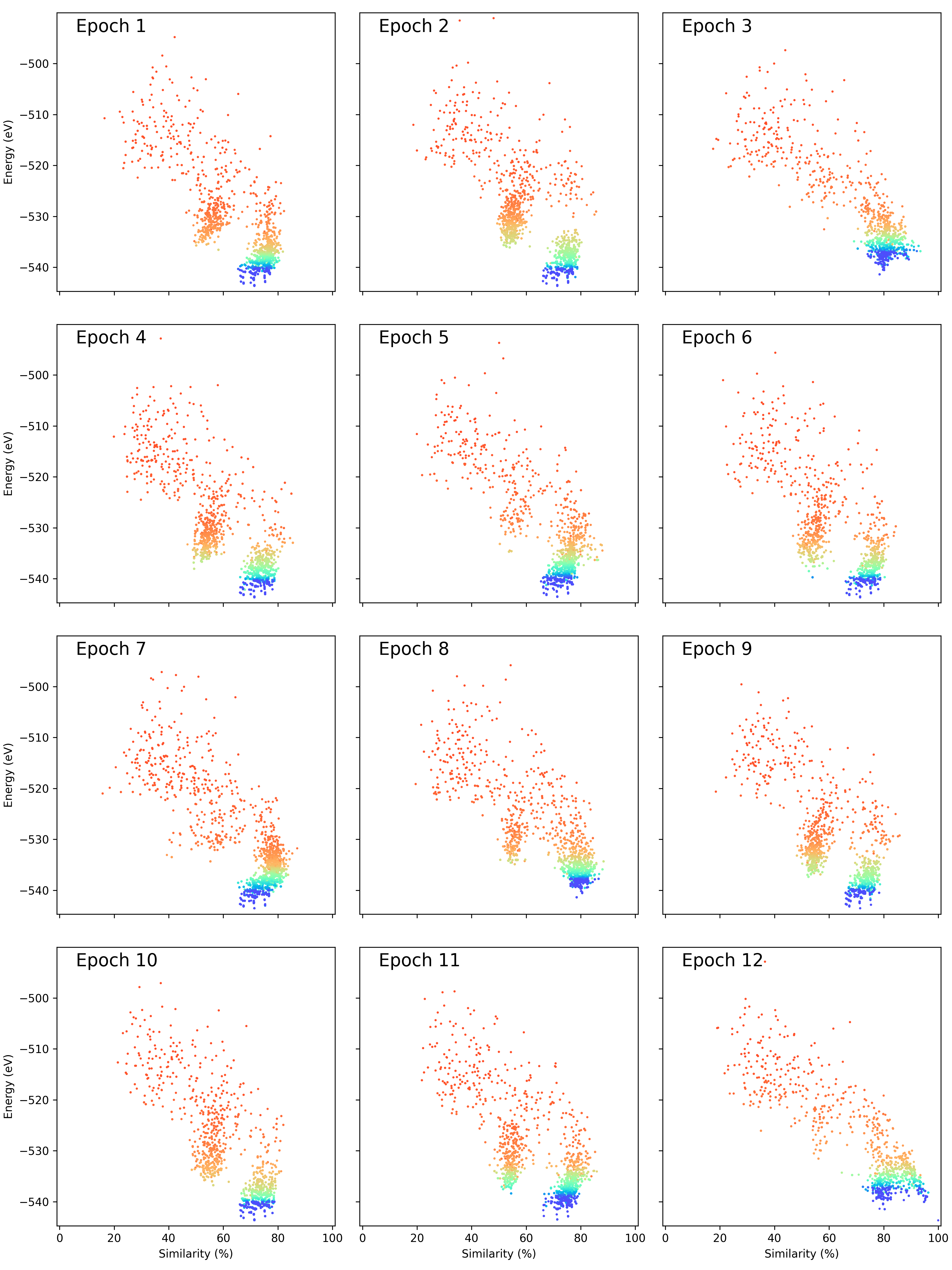
You will also get a collection of eras that are placed together on the same page so you can print them on a page together:
if get_animations = True:
This will create a video file that shows how the clusters changed over time in the population, including the offspring that are created in orange.
if get_animations_do_not_include_offspring = True:
This will create a video file that shows how the clusters changed over time in the population. This video only shows the change in the population over time without including offspring created in the video.
Troubleshooting possible issues that can arise
Here are some of the troubleshooting issue that have occurred in the past and possible troubleshooting solution to problem:
While ANALYSE CLUSTERS AND CNA PROFILES, each cluster are taking a very long time to process
I have found that sometimes the Cluster Analysed: does not show up while the program is running for some reason. However, something to check is what is being written to energy_and_GA_data.txt and CNA_Profile_data.txt in your Similarity_Investigation_Data folder and keep opening it up multiple time to see if new clusters are being written to these files.
If it is taking a while for a cluster to be written, take a look at the CNA profile that are being written to CNA_Profile_data.txt. The CNA profiles should contains many entries of signatures, like for example:
{'CNA_profile': [Counter({(4, 3, 3): 78, (4, 2, 2): 66, (5, 5, 5): 61, (3, 2, 2): 49, (2, 1, 1): 42, (5, 4, 4): 39, (3, 1, 1): 36, (2, 0, 0): 27, (4, 2, 1): 22, (3, 0, 0): 4, (1, 0, 0): 3, (4, 1, 1): 3})], 'name': 1}
You will notice that all the CNA signatures (given in brackets, e.g. (4, 3, 3)) have quite low numbers. For two atoms that are within ‘bonding distance’ of each other, the first number indicates the number of atoms that neighbour both these atoms. There are only so many atoms that can be confined near two atoms. Often this first value is between 1 to 5.
If you have entries that look more like this
{'CNA_profile': [Counter({(113, 225, 208): 4753})], 'name': 1}
where you have very large numbers in your CNA signatures, this is a sign that you have set your rCut value way to high, or somewhere in your Run_energy_vs_similarity_script.py script you have accidentally changed your rCut value to a very high value. Make sure that you set rCut to a value somewhere in between the first and second nearest neighbour values (ideally to half way between these values).